How to make a biotrace with a single match

Most intuitively we may think of ‘tracing' as a systematic inversion of a set of causal steps - the steps lead from an initiating ‘source' to an endpoint observation so the complete inversion corresponds to the identification of a source based on downstream evidence.

In the special case of biotracing the steps are often the elementary processes in a food chain that facilitate the spread of contamination and the source identification concerns the origin of particular populations of pathogenic bacteria or other harmful agents in food. However in many applications, particularly forensic sciences, a causal approach is never established and the stepwise inversion process is rejected in favour of a ‘match'. In this context a match, strictly a type match, corresponds to the coincident observation of a particular marker, with a particular value, at two distinct space-time points. Based on the discriminative properties of the marker the match is used to infer a connection between the two points and, in conjunction with known time ordering, this is used to indicate belief concerning the upstream source of a particular downstream event i.e. used to establish a trace. Fingerprints or DNA evidence used in crime investigations are the most visible forms of matching but outbreak investigations often use this principle and the concept is equally relevant for food chain biotracing.

We may illustrate the matching concept, for food chain biotracing, with a very simple example - SimpleMatch. We consider an observation, at a downstream monitor in a food production chain, which is indicative of a possible hazard. The observation may lead to a variety of interventions but, crucially for matching, includes a report of some type information. The type information in the report, which could be a genotype, biotype or other marker, can be designated as "report type = x" where x is one of the known types for the marker. In the simplest model we assume that there are exactly nT types and that there is no prior information that discriminates between them. Additionally we assume that there are exactly NS possible upstream sources for the agent (strictly for the observation) and, hence, for the marker. Again we consider there is no additional information that discriminates the sources.

If we choose a source at random, from NS possible sources, the probability that it is the true cause of the observation is simply 1/NS; all sources are equally likely. However if we measure a marker with type x for the chosen source, "source type = x", we establish a ‘match' and belief about the true cause of the observation changes. Updated belief about the true cause of the observation, based on the match evidence, depends on the number of potential sources and on the number of discriminating types. Clearly if the marker was very discriminatory, nT >> 1, the match would be a strong indication that the chosen source was the actual cause of the observation.

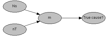
More systematically, as a first approximation, we may consider that the NS - 1 un-typed sources each have a probability, nT-1, of matching with the reported type. In this case the unknown number of un-typed sources that would produce a match, denoted m*, is distributed as p(m* | NS, nT) ~ Binomial(NS - 1, nT-1). In turn we may consider that the chosen, type matched, source is one of m = m* + 1 possible causes for the observation and therefore it is the true cause with probability m-1. Intuitively we identify the expectation of m-1, evaluated with respect to p(m | NS, nT), with a belief that the matched source is the true cause of the observation (The conditional probability for m is simply a shifted version of the conditional for m*).

This probabilistic model is easily represented as a four node belief network. In this network the node "True cause?" has states {0, 1} and the expectation of m-1 is conveniently established by the conditional probability p("True cause?" | m - 1) ~ Binomial(1, m-1). The network probabilistic models for both m and m-1 can be created as seen below:

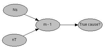
In this example a match observed at a single source, randomly selected from 101 potential sources, leads to 82% belief in true causation in the presence of 250 distinct types.

In practice this model is slightly incorrect and it overestimates the probability of true causation. More accurately the conditional probability for m, given NS, nT, is not exactly binomial because there is extra conditioning information; we know that at least one source is a match. The precise form of the conditional probability is complex but can be evaluated exactly as (see appendix)

where Q = nT-1 and the single match was obtained with a random selection. The network structure for this model is unchanged but, in HUGIN, the conditional probability table, for m, must be evaluated off-line and inserted into the net file. The corresponding belief for "True cause?" is 71%.

These numbers correspond to a famous problem in forensic science called the "Island problem" which was introduced by Eggleston (R. Eggleston, Evidence, proof and probability, Weisenfeld 1983).

The SimpleMatch network model includes very many simplifications. In particular the network treats all marker types and all un-typed sources equally, without any informative prior information, which rarely corresponds with actual beliefs. In addition the identified match, obtained from a single source chosen at random, is somewhat implausible. However this network includes many of the features that are an essential part of the matching process and provides a clear indication of the forensic approach to inference in relation to source level propositions. In SimpleMatch beliefs concerning the true cause are not strongly affected by a match when the number of types is small and beliefs about causation (guilt!) is strong for a single matched source in a small number of potential sources (suspects!). Realistic models include prior beliefs about persistent types and about source type associations and matches are identified from database records or from systematic search strategies. These extensions, in relation to source tracing in food chain systems, are the subject of EU IP BIOTRACER.

Appendix: The conditional probability for the number of potential causes for a typed report.

We consider irreversible transport of agents, that each carry a marker, from a set of NS > 0 potential sources to a report point. A report indicates the marker has a particular type, x, which is one of nT known types. The number of sources that have type x, 1 ? m ? NS, is uncertain. We assume that each source of agents has a single marker type and that the marker, and hence the report, arises from a single source.

Then, given m, the probability that the marker in the report is type x is p("report type = x" | m, NS) = m/NS. Additionally if we chose a source at random and establish type information we have p("source type = x"| m, NS) = m/NS. These probabilities are independent so that

p("report type = x", "source type = x" | m, NS) = (m/NS)2

Then Bayes' theorem gives

p(m | "r = x", "s = x", NS, nT) = C-1 p("r = x", "s = x" | m, NS) p(m | NS, nT)

where we have abbreviated the propositions and the normalizing term is C = p("r = x", "s = x"| NS, nT). Assuming that all sources are equivalent the prior probability for m is p(m | NS, nT) = Binomial(Ns, Q) where Q = nT-1. Substituting gives

Normalization, over m = 1, NS, gives C = (1 + Q(NS-1)).

---